 在几何上依据以O为中心的单位圆可以构造角θ的很多三角函数
几个三角函数的图形,分别为正弦、余弦、正切、余切、正割、余割和正矢。配色与上图相同
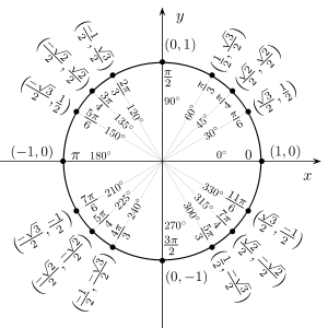 单位圆的角度
在数学中,三角恒等式是对出现的所有值都为实变量,涉及到三角函数的等式。这些恒等式在表达式中有些三角函数需要简化的时候是很有用的。一个重要应用是非三角函数的积分:一个常用技巧是首先使用使用三角函数的代换规则,则通过三角恒等式可简化结果的积分。
为了避免由于 的不同意思所带来的混淆,我们经常用下列两个表格来表示三角函数的倒数和反函数。另外在表示余割函数时,'
 '有时会写成比较长的'
 '。
'。
不同的角度度量适合于不同的情况。本表展示最常用的系统。弧度是缺省的角度量并用在指数函数中。所有角度度量都是无单位的。另外在计算机中角度的符号为D,弧度的符号为R,梯度的符号为G。
相同角度的转换表
| 角度单位 |
值
|
计算机中代号
|
| 转
|

|

|

|

|

|

|

|

|
无
|
| 角度
|

|

|

|

|

|

|

|

|
D
|
| 弧度
|
|

|

|

|

|

|

|

|
R
|
| 梯度
|

|

|

|

|

|

|

|

|
G
|
基本关系[编辑]
 三角函数间的关系,可分成正函数和余函数
毕达哥拉斯三角恒等式如下:

|

|

|
由上面的平方关系加上三角函数的基本定义,可以导出下面的表格,即每个三角函数都可以用其他五个表达。(严谨地说,所有根号前都应根据实际情况添加正负号)
| 函数
|

|

|

|

|

|
|

|

|

|

|

|

|

|

|

|

|

|

|

|

|

|

|

|

|

|

|

|

|

|

|

|

|

|

|

|

|

|

|

|

|

|

|

|

|

|

|

|

|
其他函数的基本关系[编辑]
正矢、余矢、半正矢、半余矢、外正割用于航行。例如半正矢可以计算球体上的两个点之间的距离,但它们不常用。
| 名称
|
函数
|
值[1]
|
| 正矢, versine
|


|

|
| 余的正矢, vercosine
|

|

|
| 余矢, coversine
|


|

|
| 余的余矢, covercosine
|

|

|
| 半正矢, haversine
|

|

|
| 余的半正矢, havercosine
|

|

|
半余矢, hacoversine
cohaversine
|

|

|
余的半余矢, hacovercosine
cohavercosine
|

|

|
| 外正割,exsecant
|

|

|
| 外余割,excosecant
|

|

|
| 弦函数, chord
|

|

|
纯虚数指数函数,
cosine and imaginary unit sine
|

|

|
| 辐角,Argument
|

|

|
对称、移位和周期[编辑]
通过检视单位圆,可确立三角函数的下列性质:
当三角函数反射自某个特定的 值,结果经常是另一个其他三角函数。这导致了下列恒等式:
反射于
|
反射于
|
反射于
|
反射于
|

|

|

|

|
移位和周期[编辑]
通过旋转特定角度移位三角函数,经常可以找到更简单的表达结果的不同的三角函数。例如通过旋转 、和弧度移位函数。因为这些函数的周期要么是要么是,新函数和没有移位的旧函数完全一样。
| 移位
|
移位
|
移位
|
移位
|
| 和的周期
|
, , 和的周期
|

|

|

|

|
角的和差恒等式[编辑]
 正弦与余弦的角和公式的图形证明法。使用了相似三角形的性质与三角函数的定义,强调的线段是单位长度
 正切的角和公式的图形证明法。使用了相似三角形的性质与三角函数的定义,强调的线段是单位长度。
它们也叫做“和差定理”、“和差公式”或“和角公式”。最快速简要的检定方式是使用欧拉公式[注 1]。
正弦与余弦的无限多项和[编辑]


这里的" "意味着索引
 遍历集合
遍历集合 的大小为
的大小为 的所有子集的集合。
在这两个恒等式中出现了在有限多项中不出现的不对称:在每个乘积中,只有有限多个正弦因子和余有限多个余弦因子。
如果只有有限多项 是非零,则在右边只有有限多项是非零,因为正弦因子将变为零,而在每个项中,所有却有限多的余弦因子将是单位一。
正切的有限多项和[编辑]
设 ,对于
,对于 。设
。设 是变量
是变量 ,,
,, 的次基本对称多项式。则

项的数目依赖于 。例如,
。例如,

并以此类推。一般情况可通过数学归纳法证明。
多倍角公式[编辑]
 是次切比雪夫多项式 是次切比雪夫多项式
|

|
 是次伸展多项式 是次伸展多项式
|

|
棣莫弗定理, 是虚单位 是虚单位
|

|
![{\displaystyle 1+2\cos x+2\cos 2x+2\cos 3x+\cdots +2\cos(nx)={\frac {\sin \left[\left(n+{\frac {1}{2}}\right)x\right]}{\sin {\frac {x}{2}}}}}](https://wikimedia.org/api/rest_v1/media/math/render/svg/24878792536d71a9c5b5053515b405de2af551c9) 。
。
(这个 的函数是狄利克雷核。)
双倍角、三倍角和半角公式[编辑]
这些公式可以使用和差恒等式或多倍角公式来证明。
|
|
弦 |
切 |
割
|
| 双倍角公式
|
正
|

|

|

|
| 余
|

|

|

|
| 降次公式
|
正
|

|

|
|
| 余
|

|

|
|
| 三倍角公式
|
正
|

|

|

|
| 余
|

|

|

|
| 半角公式
|
正
|

|

|

|
| 余
|

|

|

|
n倍角公式[编辑]
参见正切半角公式,它也叫做“万能公式”。
其他函数的倍半角公式[编辑]
- 正矢

- 余矢

幂简约公式[编辑]
从解余弦二倍角公式的第二和第三版本得到。
| 正弦
|
余弦
|
其他
|
|
|
|

|

|

|

|

|

|

|

|

|

|
|
|
余弦
|
正弦
|
| 如果是奇数
|
![{\displaystyle \cos ^{n}\theta ={\frac {2}{2^{n}}}\sum _{k=0}^{\frac {n-1}{2}}{\binom {n}{k}}\cos {[(n-2k)\theta ]}}](https://wikimedia.org/api/rest_v1/media/math/render/svg/c7d3151596cd1afb5389c1566d5cbe8c51523ab3)
|
![{\displaystyle \sin ^{n}\theta ={\frac {2}{2^{n}}}\sum _{k=0}^{\frac {n-1}{2}}(-1)^{\left({\frac {n-1}{2}}-k\right)}{\binom {n}{k}}\sin {[(n-2k)\theta ]}}](https://wikimedia.org/api/rest_v1/media/math/render/svg/71aeee70c9d36436ed2293c9d10d931ac3bf1635)
|
| 如果是偶数
|
![{\displaystyle \cos ^{n}\theta ={\frac {1}{2^{n}}}{\binom {n}{\frac {n}{2}}}+{\frac {2}{2^{n}}}\sum _{k=0}^{{\frac {n}{2}}-1}{\binom {n}{k}}\cos {[(n-2k)\theta ]}}](https://wikimedia.org/api/rest_v1/media/math/render/svg/313e388dfc8ef99160a6f1f04286f107bc96aa1d)
|
![{\displaystyle \sin ^{n}\theta ={\frac {1}{2^{n}}}{\binom {n}{\frac {n}{2}}}+{\frac {2}{2^{n}}}\sum _{k=0}^{{\frac {n}{2}}-1}(-1)^{\left({\frac {n}{2}}-k\right)}{\binom {n}{k}}\cos {[(n-2k)\theta ]}}](https://wikimedia.org/api/rest_v1/media/math/render/svg/450f6c0089bc8c2f424338bfd77e2efddf1f2cef)
|
数值连乘[编辑]
 [2]
[2]
 [2]
[2]
 ,
, ,
,
 ,
, ,
,
 ,
, ,
,
常见的恒等式[编辑]
积化和差与和差化积恒等式[编辑]
数学家韦达在其三角学著作《应用于三角形的数学定律》给出积化和差与和差化积恒等式。积化和差恒等式可以通过展开角的和差恒等式的右手端来证明。

| 积化和差 |
和差化积
|

|

|

|

|

|

|

|

|
平方差公式[编辑]


(可借由积化和差公式+2倍角公式推导而来)
其他恒等式[编辑]
- 如果
 ,
,
- 那么


- 如果
 ,
,
- 那么


- 如果
 ,
,
- 那么


托勒密定理[编辑]
- 如果
 (半圆)
(半圆)
- 那么:

(前三个等式是一般情况;第四个是本质。)
三角函数与双曲函数的恒等式[编辑]
利用三角恒等式的指数定义和双曲函数的指数定义即可求出下列恒等式:


所以


下表列出部分的三角函数与双曲函数的恒等式:
| 三角函数
|
双曲函数
|

|

|

|

|

|

|

|

|

|

|

|

|


线性组合[编辑]
对于某些用途,知道同样周期但不同相位移动的正弦波的任何线性组合是有相同周期但不同相位移动的正弦波是重要的。在正弦和余弦波的线性组合的情况下,我们有

这里的

这个公式也叫辅助角公式或李善兰公式。更一般的说,对于任何相位移动,我们有

这里

而

反三角函数[编辑]


无限乘积公式[编辑]
为了用于特殊函数,有下列三角函数无穷乘积公式[3][4]:
微积分[编辑]
正弦(蓝色)、正弦的微分(橘色),其中,正弦的微分正好是余弦。
余弦(蓝色)、余弦的微分(橘色),其中,余弦的微分正好是正弦的对x轴的镜射。
在微积分中,下面陈述的关系要求角用弧度来度量;如果用其他方式比如角度来这些关系会变得更加复杂。如果三角函数以几何的方式来定义,它们的导数可以通过验证两个极限而找到。第一个是:

可以使用单位圆和夹挤定理来验证。如果用洛必达法则来证明这个极限,那也就用这个极限证明了正弦的导数是余弦,并因此在应用洛必达法则中使用正弦的导数是余弦的事实,就是逻辑谬论中的循环论证了。第二个极限是:

使用恒等式 验证。已经确立了这两个极限,你可以使用导数的极限定义和加法定理来证明
 和
和 。如果正弦和余弦函数用它们的泰勒级数来定义,则导数可以通过幂级数逐项微分得到。

结果的三角函数可以使用上述恒等式和微分规则来做微分。

在三角函数积分表中可以找到积分恒等式。
三角函数(正弦和余弦)的微分是同样两个函数线性组合的事实在很多数学领域包括微分方程和傅立叶变换中是重要的基本原理。
指数定义[编辑]
| 函数
|
反函数
|

|

|

|

|

|

|

|

|

|

|

|

|
|
|
|

|

|
|
|
|

|

|

|

|

|

|
参考文献[编辑]
- ^ Abramowitz and Stegun, p. 78, 4.3.147
- ^ 2.0 2.1 苏学孟. 求三角函数乘积的常用方法. 中学数学教学. 1995, (6) [2014-12-27]. (原始内容存档于2014-12-27).
- ^ Abramowitz and Stegun, p. 75, 4.3.89–90
- ^ Abramowitz and Stegun, p. 85, 4.5.68–69


![{\displaystyle \sin n\theta =\sum _{k=0}^{n}{\binom {n}{k}}\cos ^{k}\theta \,\sin ^{n-k}\theta \,\sin \left[{\frac {1}{2}}(n-k)\pi \right]=\sin \theta \sum _{k=0}^{\lfloor {\frac {n-1}{2}}\rfloor }(-1)^{k}{\binom {n-1-k}{k}}~(2\cos \theta )^{n-1-2k}}](https://wikimedia.org/api/rest_v1/media/math/render/svg/30a3575f39e74314218d2d046b50210fc2834b8a)
![{\displaystyle \cos n\theta =\sum _{k=0}^{n}{\binom {n}{k}}\cos ^{k}\theta \,\sin ^{n-k}\theta \,\cos \left[{\frac {1}{2}}(n-k)\pi \right]={\frac {1}{2}}\sum _{k=0}^{\lfloor {\frac {n}{2}}\rfloor }(-1)^{k}{\frac {n}{n-k}}{\binom {n-k}{k}}~(2\cos \theta )^{n-2k}}](https://wikimedia.org/api/rest_v1/media/math/render/svg/4aab0b9f9ec4bc519564a1720f9d1e10338c0c2f)
![{\displaystyle \tan n\theta ={\frac {\displaystyle \sum _{k=1}^{\left[{\frac {n}{2}}\right]}(-1)^{k+1}{\binom {n}{2k-1}}\tan ^{2k-1}\theta }{\displaystyle \sum _{k=1}^{\left[{\frac {n+1}{2}}\right]}(-1)^{k+1}{\binom {n}{2(k-1)}}\tan ^{2(k-1)}\theta }}}](https://wikimedia.org/api/rest_v1/media/math/render/svg/a03b0563027ebb58ac7816288c76ead0dc0ba445)


![{\displaystyle |\sin x|={\frac {1}{2}}\prod _{n=0}^{\infty }{\sqrt[{2^{n+1}}]{\left|\tan \left(2^{n}x\right)\right|}}}](https://wikimedia.org/api/rest_v1/media/math/render/svg/71abcbf6e9d8704e6030ef84b53d6de4a37681ce)
